An algorithm to detect chords
I started the summer 2024 with a desire to learn bossa nova music on guitar. I ended that year trying to create a codebase to help me identify notes and chords on guitar. And I am doing so with the dream of creating a musical AI assistant to help me learn how to improvise music like the professionals. How’s it going? I have a system for labeling sound data and creating models to predict the labels using the sound’s frequency spectrum.
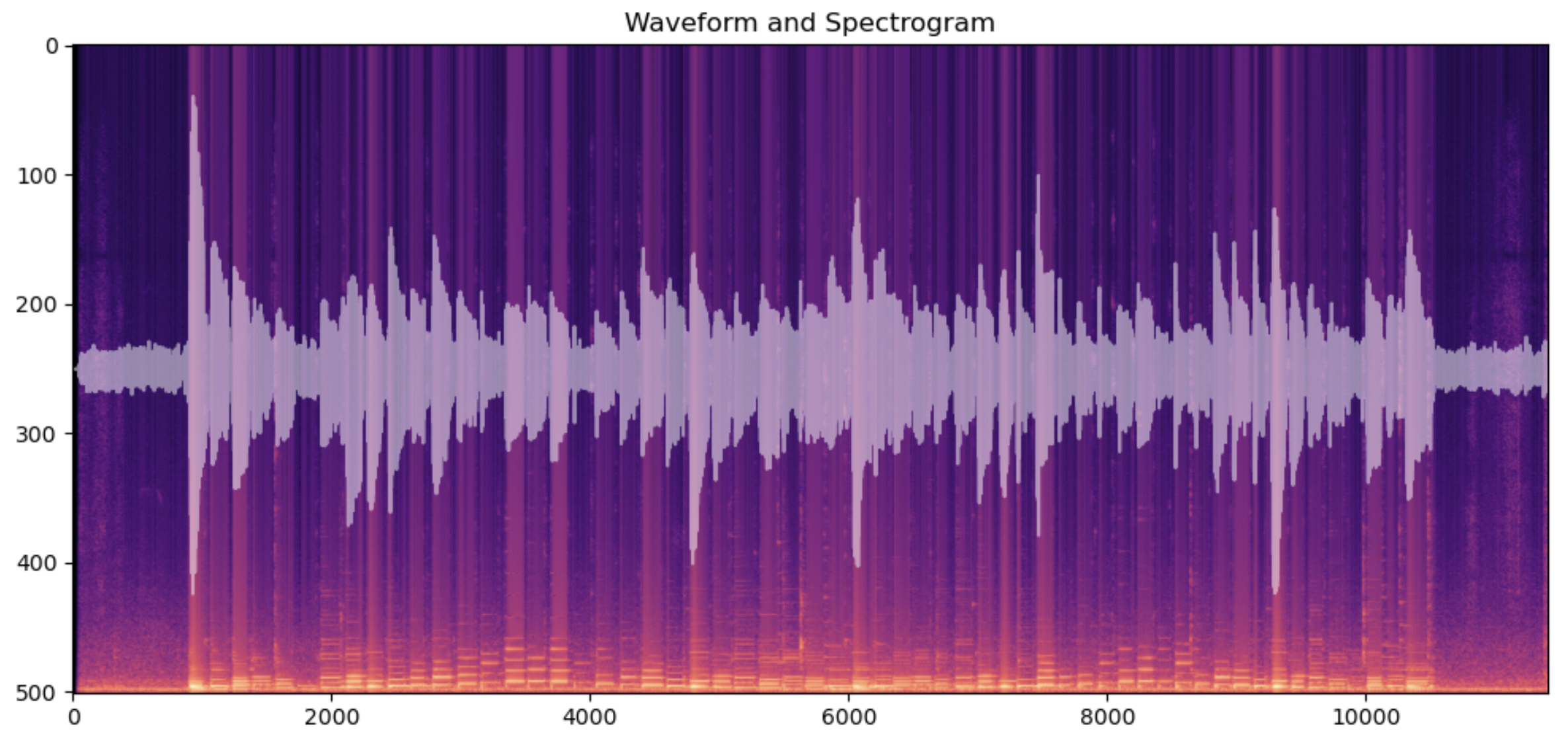
Here I have played a G major scale, two octaves, up and down twice. The light colored spikes around the centerline are the waveform. The colorful bands in the background are a spectrogram. Spectrogram is an image created by a series of fourier transforms on windows of the sound data. This is the short time fourier transform (STFT). This transformation takes a vector of sound data and sweeps a window function over it. This window function outputs a vector of numbers representing how much each frequency is present in the window. Which frequencies? They are a series of discrete waves that fit inside the window. So their frequencies are integer multiples of the fundamental frequency, the one whose wave fit exactly one period inside the window. The calculation of these fourier coefficients is sped up by a technique discovered by John Tukey known as the fast fourier transform.
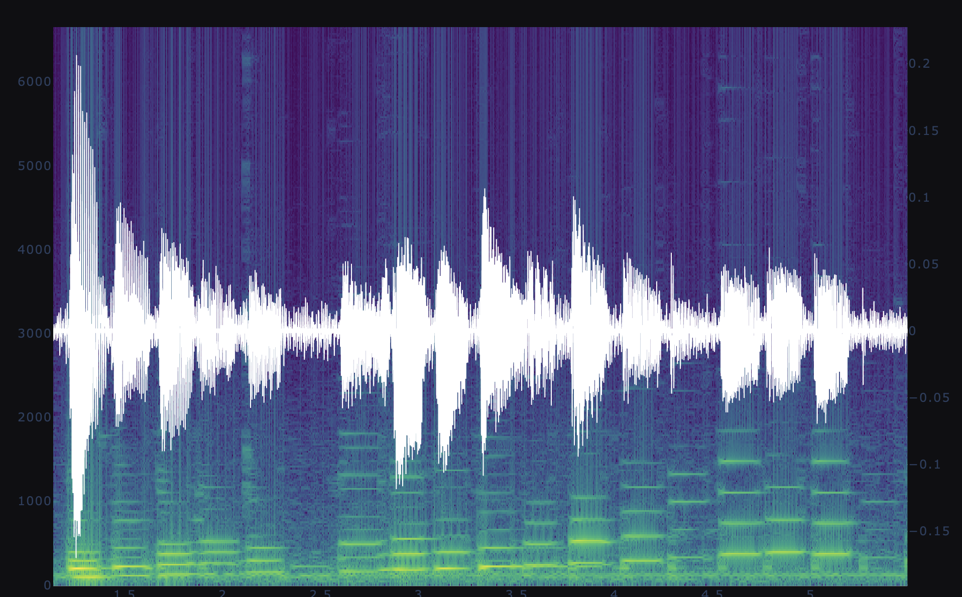
The result is a vector of values the correspond to the presence of a frequency in the window. By sweeping the fourier transform window over the sound data, we get 2 dimensional data. One dimensions is the time that is tied to the window. The other dimension is the frequency value of each component in the Fourier series. Since the data is now 2 dimensional, so it is natural to plot it as a heatmap image. The scale used below is viridis, giving a blue to green to yellow color based on a pixel’s value. This image data is what will be used to predict the label of the sound.
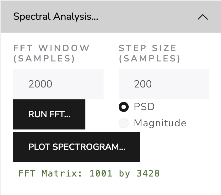
Parameters of the short time fourier transform (STFT)
G major scale, ascending two octaves, then descending two diatonic steps to E. Sample rate 44100 samples per second, Fourier gaussian window size 2000 samples with sigma=1000, hop size 200 samples.
Using python Dash, I set up a visual interface where I can select regions of the sound and label them. I used my ear to identify the notes and label them manually. The interface allows me to select a region of time, play it to ensure I’ve selected the correct area, and enter a label and save it to a json file on the server. This was my first attempt. In subsequent attempts I split and clustered the sounds so increase the efficiency of labeling.
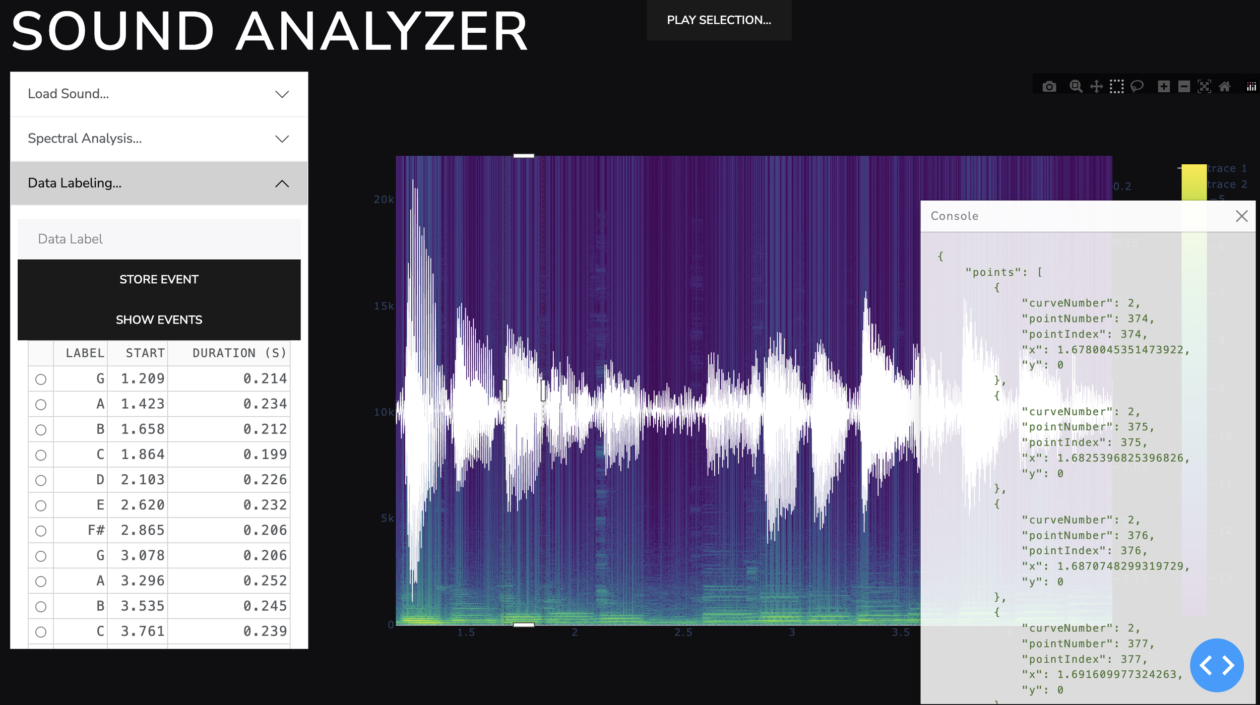
The labeling interface of my custom sound analyze app.
I reduced the spectra dimension from 1001 to 16 using a basic linear technique called principal component analysis (PCA). This produces variance maximizing components that can reconstruct the original spectra with some error. The components are what I will use to cluster the sounds by similar harmonic content. This step was not completely necessary, but in reducing the dimension of the predictor space, it reduced the time required to fit the classification models at the end.
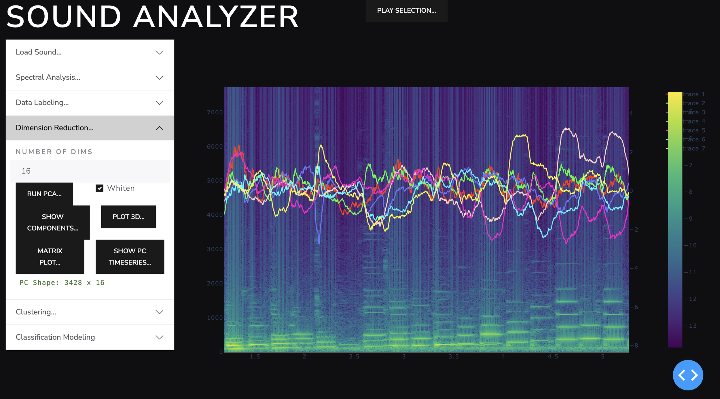
a time series of the principal components of the frequency spectra. These component values through time were what I used to cluster the sounds.
The clustering algorithm chosen was Agglomerative clustering. Kmeans did not do a good job, and agglomerative worked much better. Additional algorithms were not tested. The UI is built to allow user to click through the individual regions of time identified by the clustering algorithm. Because the clusters could oscillate between different clusters as points when notes changed, I also included a temporal-smoothing algorithm for cluster label. It turned out that sometimes the individual cluster was just noise. Some clusters showed specific notes often in multiple octaves. The note G appeared in 3 octaves, the rest of the notes appear in two different octaves. It was pleasing that the unsupervised algorithm (clustering) did a good job at putting together things were fundamentally similar but not exactly the same.
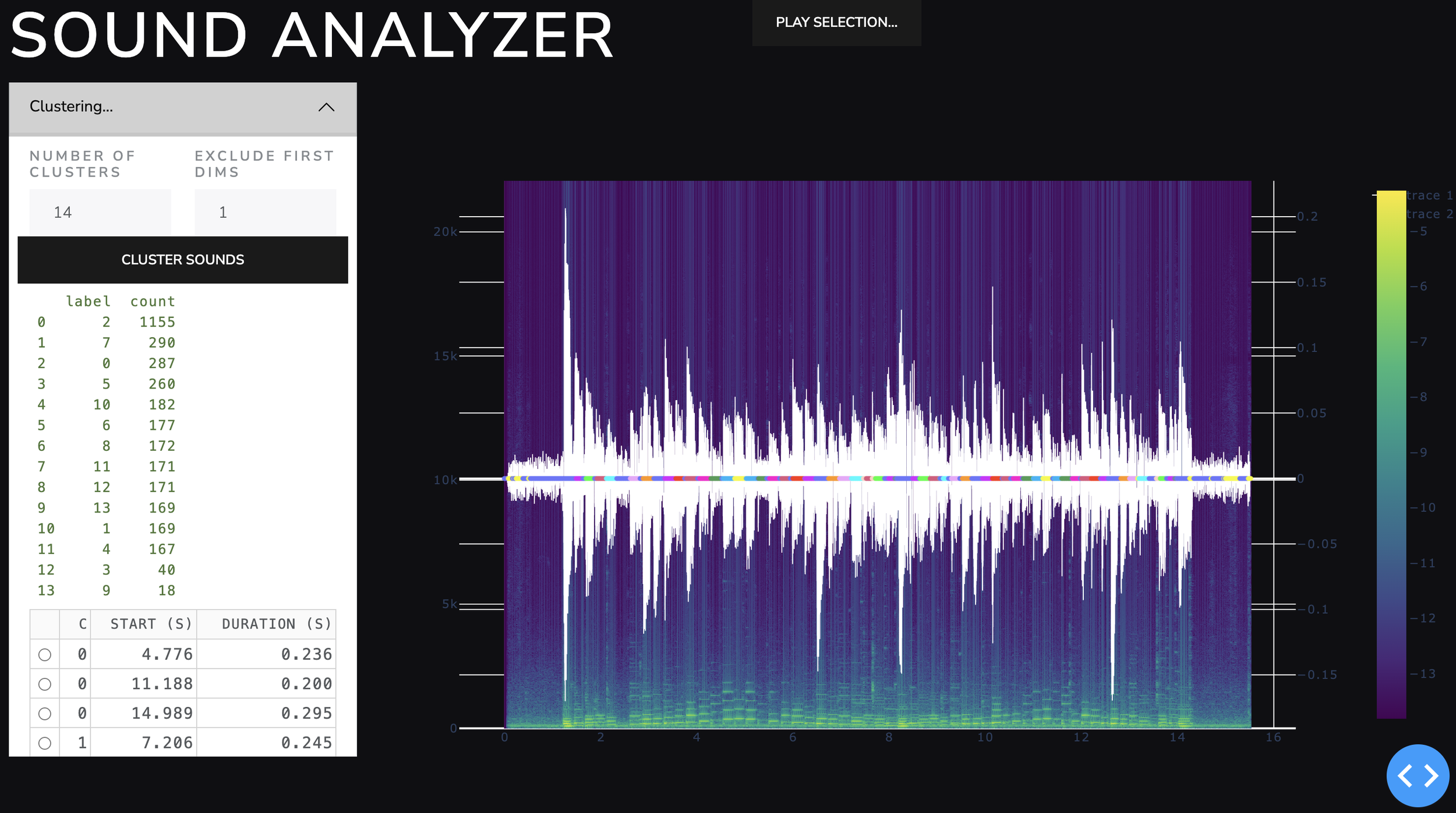
The spectrogram with sound wave form overlayed. Harmonic clusters shown as colored dots at the midline of the graph.
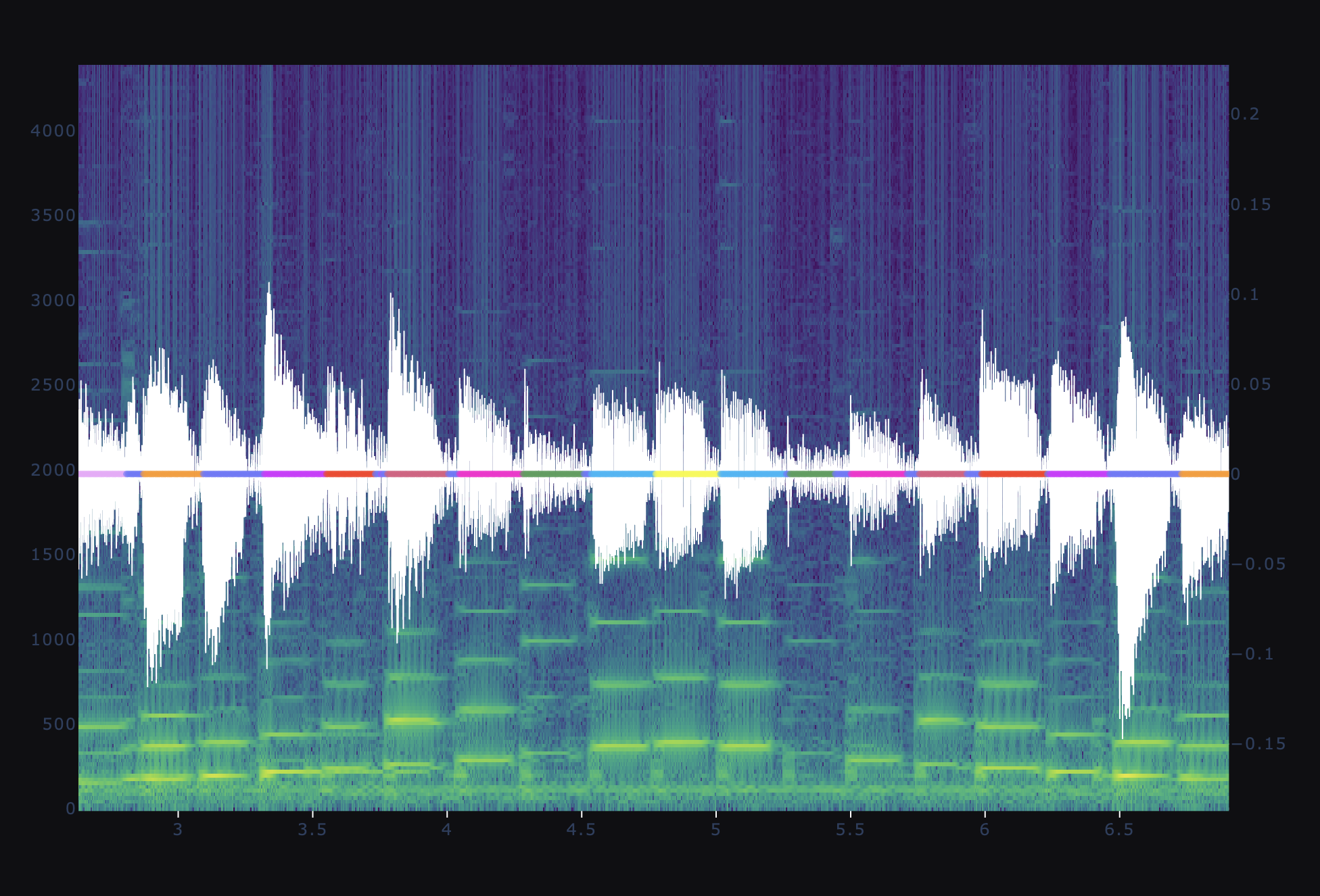
Part of the G major scale. Cluster labels shown as colors are symmetric about the highest note, G, as expected.
Now I needed to employ a supervised algorithm, an algorithm that is trained to predict a target. I had clusters which contained notes of similar harmonic content. But I wanted an algorithm that could detect and name specific content in sound.
Below is the prediction made by a random forest classifier trained to predict note label given spectrum principal components. The prediction probability is highest for the notes the model is trained on. The subsequent note that were not included in the training data show lower predicted probability. Additional training on more notes, would improve overall ability to identify notes.
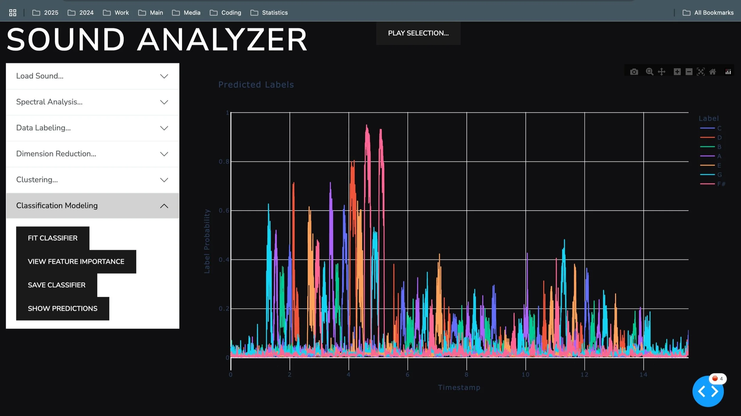
Note probability predicted by a random forest classifier trained to predict note label given spectrum principal components.
But, I wanted to detect notes and chords. Would individual note models be enough to detect chords? Would there be any advantage to building models for chords based on playing those chords? Or would composable models that detect individual notes be enough to name the chord being played? There are areas of research that I continue to work on using this sound analyzer application.
The code I created to perform this analysis and user interaction is on my github: